SEM Spectrum Data Analysis and MATLAB code

The instructions that are provided below are specific to obtain and save EDS x-ray spectrum data to an '*.xls' excel file so that the spectrum can be plotted in MATLAB along with calculating the K-Alpha values of the particular element.

An elemental mapping can be obtained using the 'HYPERMAP' option in the edx application of the SEM. After the application has completed acquiring enough counts to quantify elements, the spectrum could be calculated using manually selecting a specific region using the option highlighted in the red box below. All the options mentioned below can be seen in the bottom right corner of the edx application.

Selecting the option in the red box, allows you to select the region of the captured image to obtain the spectrum from. In general, the whole image is selected to scan for the spectrum.

The option boxed below automatically calculates the 'Maximum Pixel Spectrum' that is the spectrum of the full image with the element of the highest peaked counts. Such an option is beneficial when we calculate the spectrum of a sample with a specific primary element.

Once the option is selected the progress bar, shown below, should indicate the calculation of the high pixel spectrum,

After the spectrum has been successfully calculated using either method, click on the 'spectrum' tab to view the spectrum. Then click on the periodic table icon which will display a periodic table of elements. The 'Auto' button on the bottom right corner of the periodic table will display the elements that are present in the spectrum. Manually selecting the spectrum will show you a series of elements that might or might not be present; Check the peaks of the elements by zooming into the spectrum and thereby determine the presence of the element in the sample. Using the 'Maximum Pixel Spectrum', the 'Auto' button will only show one element in the spectrum that is primarily present. Aditional elements can be selected according to peak heights. It is important to press 'Auto' before quantifying data.

The name of the spectrum could be changed for convenience, by double-clicking the name below the spectrum, as shown in the image below;

Prior to saving the spectrum data, the spectrum should be quantified using the 'quantify' button shown below;

Once the spectrum is quantified, the arrow button to the right side of the tabs, shown below, gives you the option to save the raw spectrum data.

Clicking the 'Save' button prompts a dialog to choose a location and filename to save the raw spectrum data. It also provides the option to save the spectrum in three different data formats, that is .xls, .txt and .spx as shown below. The format '.spx' is the data file accepted by the edx application 'Espirit 1.9'. The format '.xls' is the excel data file with the spectrum data that is accepted by the MATLAB code. It is recommended to save the data using both .spx and .xls formats.

Once the excel file has been created through the edx application 'espirit', simply open the '*.xls' excel data file to make sure the file is not corrupt. Almost every time, the data file is corrupt and you will be prompted to recover data as shown below. Click 'yes' and no data will be altered. 

Click 'Ok' to the message followed by clicking 'yes' to recover data in the previous message. The excel data file with the spectrum data can be seen after.

Even though no changes were made to the data file, SAVE the file with the "recovered" data so that MATLAB can read the spectrum data without any complications. The MATLAB code for the SEM spectrum and the excel X-ray Characteristic line data file can be found in the google drive link provided below (Log-in using your Siena email);

https://drive.google.com/drive/folders/0B2ACmmug9K_UY2h1ejJNZVdsU0k?usp=sharing

[Revised] XRF Spectrum Data Analysis and MATLAB code

The MATLAB code to plot the X-ray spectrum, to find the K-Alpha value of the element and to plot the Moseley's Stright line has been altered and upgraded to accept data files that are directly taken for the XRF HD prime. The procedure to take the spectrum data from the HD prime and convert it into an excel data file is explained in the previous 'XRF HD Prime Spectrum Data Analysis' blog post i.e found at;

https://saintcenter2017.blogspot.com/2017/06/xrf-hd-prime-spectrum-data-analysis.html

Once the excel file has been created through the HD data viewer, simply open the '*.csv' excel data file to make sure the file is not corrupt. Some times, the data file is corrupt and you will be prompted to recover data. Click 'yes' and no data will be altered. Even though no changes were made to the data file, SAVE the file you opened and 'recovered corrupt data'. 

Note; The X-ray Characteristic line data file that is named 'Xrayline.xlsx' , should not be renamed and should be placed in the same location as the MATLAB code file. The MATLAB code that is named 'XRFSpectrum.m' should not be renamed either. The XRF HD prime data could be placed in a different folder since you are prompted to select the data file within the script.

Simply run the MATLAB code and follow the instructions to input and select the information that is required. It is important to accurately insert the Atomic symbol of the element in the correct format when prompted in MATLAB. The First letter of the symbol is UpperCase and the rest lowercase. Example; Iron would be 'Fe', NOT 'FE' or 'fe'. Vanadium would be 'V' and NOT 'v'.

The MATLAB code for the XRF Spectrum and the excel X-ray Characteristic line data file can be found in the google drive link provided below (Log-in using your Siena email);

https://drive.google.com/drive/folders/0B2ACmmug9K_UY2h1ejJNZVdsU0k?usp=sharing

The effect on the magnetic field on the image of SEM

"Various reasons of the distortion is based on measurements of the periodic deformations of the images for different electron beam energies and working distances between the microscope final aperture and the specimen. Using the SEM images, a direct influence of alternating magnetic field on the electron beam was distinguished."

The direct electron beam deflection depends on the magnetic field magnitude and the working distance, i.e. distance between the final aperture of the electron gun and the specimen.

Paper that explains the measurement of a B-field in a SEM;

http://www.sciencedirect.com/science/article/pii/S0968432808000188

Expression states to calculate the magnetic field;

Where Bx and By are two orthogonal components of magnetic field vector B, e is electron charge, E is energy of electrons, Me is relativistic electron mass, Vx0 and Vy0 are orthogonal components of initial electron velocity (initial, i.e. at working distance=0) parallel to Lorentz force direction, dx0 and dy0 are orthogonal components of initial electron beam deflection.

Quantum Dot Testing

Quantum Dot Testing      

Why Test Quantum Dots?

Quantum dots have demonstrated extensive potential in biomedical applications due to the combination of their unique photophysical properties, and the ability to render them biocompatible and specific by conjugation to various biomolecules. Their use is underway in various immunological and molecular assays for different pathogens and biomarkers. For the clinical laboratory, quantum dots are used as tools for ultrasensitive multiplexed diagnostics. Additionally, the combined utilization of quantum dots with their unique optical properties and microfluidics would aid the development of sensitive bioanalysis systems, and aid in the efforts towards their use for point-of-care testing, which would allow the movement of testing processes closer to patients in remote locations with limited infrastructure and decrease reliance on central laboratories. Also, point-of-care testing would support field testing in disease outbreak areas. Commercial availability of various types of quantum dots is substantially increasing and a large body of successful studies of clinical utility has already built up. These factors are highly conducive and indicative of a more significant role of quantum dots in the future of bioanalysis. The next decade in the world of medicine, biology, and physics we can expect to see a noticeable advancement in the use of quantum dots.

For our first data collection we found the following values:

560 nm

The Wavelengths ranged between 380nm-900nm

The Absorbance hovered around 3 until it hit 530nm, then it decreased to almost zero until 600nm, and then it increased back up to 3

*Working on getting a picture of the spectrum to place here*

(Here we will insert more data on our quantum dots when we conduct more experiments)

Below are pictures and descriptions of how we conducted our experiment.

Above is a picture of our set up with the lights on to see how our experiment was actually conducted. Here we can see one of our Quantum Dot samples placed on a lit UV LED Flashlight. We then held up a fiber optic cable near the quantum dots and placed the other end into the SpectroVis Plus. The SpectroVis Plus was then plugged into a laptop where we could see the spectrum produced there.  When we were ready to conduct an experiment we would turn the lights off, lower the brightness of the laptop we were using and only turn on the UV LED Flashlight. This would reduce as much light interfering with our quantum dots as possible and only have our sample exposed to UV light.

Above is what it looked light when we turned off all the lights. As we can see, we did a great job at reducing the most amount of light as possible when conducting the experiment. Once the lights were off we were able to turn on the UV Flashlight, hold the fiber optic cable up to the quantum dots, turn on the spectrometer, and click run on the laptop to run the sample. Data collections usually took less than a minute to collect all the necessary data needed for each sample. 

Above is one of our Quantum Dot samples placed onto a UV LED Flashlight. This is how we exposed light to our quantum dot samples and collected data.

Above is a picture of the portable UV-Vis Spectrometer we used titled SpectroVis Plus. This was a great way to start our spectrometer research and familiarize ourselves with how to collect data from a spectrometer. We wanted to use this instrument before using the larger Agilent Cary 100 Ultraviolet-Visible (UV-Vis) Spectrometer in the SAInT Center. Using it is simple in the sense that you just need to place your sample either in a test tube or cuvette and place it in the square slot on the top of the spectrometer. In the picture above we were studying an already prepared sample given to us by the chemistry department and tried running a sample and collecting data.

Above is a picture of a Vernier LabQuest Device that we used to look at the spectrum our samples produce. We can plug this instrument into the SpectroVis Plus and collect data that way.

Above is a picture of one of our research students Cham. Here he is working with a portable UV-Vis Spectrometer plugged into a LabQuest. We ran some samples through this to familiarize ourselves with the data collecting process, and how to use a UV-Vis.

Nickel Sample

Nickel Sample

The results from the SEM for the Nickel Sample which is one of six samples in the stage provided by Dr. McColgan and Dr. Hassel. The elemental map of the sample and a spectrum of elements present in the sample was obtained from the microscope. The spectrum is quantified to get a percentage composition of the elements that were detected in the sample.

The elemental map of the sample with a specific color for each element is shown below;

The spectrum of the elements that were counted is shown in the image below; 

Image of the section in the sample that was used to find the elemental composition is shown below;

The percentage composition of each element that was considered to be primarily present in the sample is shown in the table below. Elements such as Carbon and Oxygen were neglected since they are abundant in the air or present in the stage where the sample was placed.

Element	AN	series	[wt.%]	[norm. wt.%]	[norm. at.%]	Error in wt.% (1 Sigma)
Chromium	24	K-series	0.867162	0.896885	1.011241	0.049409
Nickel	28	K-series	95.81883	99.10312	98.98876	2.389692
		Sum:	96.68599	100	100

The peak energy values of each of the elements in samples that were primarily presented can be seen in the horizontal axis of the spectrum shown above. The peak values were manually recorded as listed below;

Nickel (Z - 28): 0.749 keV, 0.854 keV, 7.480 keV (K-Alpha), 8.264 keV (K-Beta)

Chromium (Z - 24); 5.416 keV (K-Alpha)

The actual K-Alpha and K-Beta values for elements can be looked up using the Characteristic X-ray Line Energies table attached in the posts of the other samples including the stage of all the samples that was analyzed.

 Below is the data we collected using the HD Prime X-Ray Flourescence (XRF) Analyzer:

Zirconium Sample

Zirconium Sample

Here is a blog that consists our data about the Zirconium (Zr) Sample taken under the Scanning Electron Microscope (SEM). Dr. Hassel and Dr. McColgan provided us with 3 stages that each consisted of 6 different element samples in them. This is the data we collected when we studied the Zirconium Sample from these stages. Below is the data we collected:

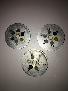
Above is a picture of the stages we used that consisted of the 6 different metal samples.

Above is the spectrum for our Zirconium Sample.

In the Zirconium Sample we found traces of Zirconium(Zr), Hafrium(Hf), and Chromium(Cr). Zirconium peaked at 0.157 keV, 2.054 keV, and 15.730 keV. For Chromium, it peaked at 0.526 keV and 5.412 keV. For Hafrium, it peaked at 1.656 keV and 7.892 keV. 

 Below is the data we collected using the HD Prime X-Ray Flourescence (XRF) Analyzer:

Vanadium Sample

Vanadium Sample

Here is a blog that consists our data about the Vanadium (V) Sample taken under the Scanning Electron Microscope (SEM). Dr. Hassel and Dr. McColgan provided us with 3 stages that each consisted of 6 different element samples in them. This is the data we collected when we studied the Vanadium Sample from these stages. Below is the data we collected:

*Note: When observing this sample we noticed that this sample charged up significantly.*

Data Number: SAInTCentr

Magnification: 2300

Accelerating Voltage: 30000 Volt

Emission Current: 85000 nA

Working Distance: 15300 um

Above is a picture of the stages we used that consisted of the 6 different metal samples.

Above is the spectrum for our Vanadium Sample.

In the Vanadium Sample we found traces of Vanadium(V), Aluminium(Al), Silicon(Si), and Sulfur(S). Vanadium peaked at 0.525 keV, 4.964 keV, and 5.428 keV. Aluminium peaked at 1.495 keV. Silicon peaked at 1.742 keV, and finally Sulfur peaked at 2.307 keV.

 Below is the data we collected using the HD Prime X-Ray Flourescence (XRF) Analyzer:

Lead Sample

Lead Sample

Here is a blog that consists our data about the Lead (Pb) Sample taken under the Scanning Electron Microscope (SEM). Dr. Hassel and Dr. McColgan provided us with 3 stages that each consisted of 6 different element samples in them. This is the data we collected when we studied the Lead Sample from these stages. Below is the data we collected:

Data Number: SAInTCentr

Magnification: 2300

Accelerating Voltage: 30000 Volt

Emission Current: 87000 nA

Working Distance: 15100 um

Above is a picture of the stages we used that consisted of the 6 different metal samples.

Here is a picture of our Research Team enjoying our time studying metal samples on the SEM. The picture is of Tristen Protzmann (left), Chamidu Warnakulasuriya (middle), and Brendan Waffle (right).

Above is the spectrum for our Lead Sample.

In the Lead Sample we found traces of Lead(Pb) and Chromium(Cr). The peaks we found were that Lead peaked at 0.278 keV, 1.835 keV, 2.335 keV, 9.179 keV, 10.544 keV, and 12.610 keV. As for the Chromium, it peaked at 0.523 keV and 5.409 keV.

 Below is the data we collected using the HD Prime X-Ray Flourescence (XRF) Analyzer:

XRF HD Prime Spectrum Data Analysis

Saving Data

The XRF HD Prime provides a variety of ways to save the quantified results from the sample which includes the full results or summarized results. Either way, the results of the spectrum which represents the counts recorded with respect to each energy (in keV) are not recorded in these files. 

Simultaneously hold the buttons 'Ctrl' + 'Shift' on the keyboard connected to the HD prime, to view the spectrum.  This will prompt a dialog to enter the expert password which will grant you access to view the spectrum along with the spectrum line for each element.

Each time the XRF quantifies a sample, a copy of the all the data related to the sample is automatically saved under one file (.hdx extension) to the folder with the date of data collection.

(Common Folder:  C:\Data\[Date of Data Collection])

A software named HD Data Viewer can be used to open such a file to view and save spectrum data. This software shows all the data including the full results, summary, a picture of the sample from the camera, and all the spectrum data, both in linear and log axes. This software is required to export the spectrum data we need to plot the spectrum in Matlab and calculate the peak values.

In HD Data Viewer;
-Import the data by clicking on the 'open' button and selecting the correct '.hdx' file.
-If the scanning information found on the bottom-left corner and the sample picture is correct, the data has been sucessfully imported.
-To view the spectrum data, click on the 'spectrum view' Tab on the top. (Ctrl + 3 for Windows PC)
-The spectrum can be viewed in Log or linear scale. The spectrum for each element listed on the right can also be viewed by simply marking the check-up box next to the particular element.
-Only the 'Raw spectrum' will be selected to export all the necessary data. 
-The drop-down menu in the 'CSV' button will provide you with the option to export the spectrum data from Low, Medium and High energies as shown below.

- Save '.csv' file to a convenient folder.
- To import data to MATLAB easily, the data table in Excel file should be Transposed.

Preparing data fro MATLAB

• Open the excel sheet exported from HD Data Viewer and select all the data.
• Simply select the first cell (A1), scroll all the way to the last cell (BZU4), Hold 'Shift' and select the last cell.
• Right click and Copy.
• Open a new blank Excel worksheet. 
• Select the First cell (A1), right click and do a 'Transpose (T)' paste.
• Save the new excel data sheet

XRF Spectrum in MATLAB

The goal is to use MATLAB to recreate the XRF spectrum, find the peak that is the highest counts and the corresponding energy that represents the K-Alpha value of the primary element.
Furthermore, we can find the counts acquired to the actual value of K-Alpha value of the element/metal.

The 'uiimport' function can be simply used in a script to prompt the user to import the data that we prepared in the previous step. The data will be already selected and ready to be placed in variables that are automatically created. 

The 'pause(time in seconds)' function is also used to give a user enough time to select data before executing the rest of the script.

Select the correct excel data file that was prepared and the data will be automatically selected. MATLAB will prompt the following dialog;

Four new variables will be created which will be seen using 4 blue underlined names. The Data Import dialog can be closed after the data was successfully imported and the rest of the code that depends on the data that was imported will be executed. 

The script that I used to plot the spectrum, find the peak and the other necessary values is shown below;

------------------------------------

prompt = 'How many Samples? ';
N = input(prompt);
Kerror = zeros(N,1);
K = zeros(N,1);
Atomic = zeros(N,1);

for i=0:N-1;
    
close all
clearvars -EXCEPT N Kerror K Atomic i

prompt = 'What is the K alpha of the primary element? ';
realalpha = input(prompt);
prompt = 'What is the Atomic Number of the primary element? ';
Z = input(prompt);

uiimport

pause(20)

LnLE=log(LESubstrateRawSpectrumCounts);
LnME=log(MESubstrateRawSpectrumCounts);
LnHE=log(HESubstrateRawSpectrumCounts);
figure(1)
plot(EnergykeV,LnLE)
title('LE')
xlabel('Energy (keV)')
ylabel('ln (Counts)')
figure(2)
plot(EnergykeV,LnME)
title('ME')
xlabel('Energy (keV)')
ylabel('ln (Counts)')
figure(3)
plot(EnergykeV,LnHE)
title('HE')
xlabel('Energy (keV)')
ylabel('ln (Counts)')

[value, location] = max(LnLE(:));
PeakCount=value
Kalpha = EnergykeV(location)

loc = find(EnergykeV>=realalpha);
LiteratureCount = LnLE(loc(1,1))
% loc2 = find(EnergykeV<=realalpha);
% LiteratureCount2 = LnLE(loc(1,1))
% AvgLiteratureCount= (LiteratureCount+LiteratureCount2)/2
Diff = abs(Kalpha-realalpha);

ind = logical(i);

Kerror(ind+1) = Diff;
Atomic(ind+1) = Z;
K(ind+1) = Kalpha;

end

figure(4)
[m,c] = polyfit(Atomic,K,1);
y = polyval(m,Atomic,c);
plot(Atomic,K,'r.'); hold on;
errorbar(Atomic, y, Kerror);
title('Mosleys Plot')
xlabel('Atomic Number')
ylabel('Energy (keV)')

------------------------------------
The script also produces the Mosley's Plot from the Kalpha and atomic numbers of all the samples that are inserted.

Manganese Sample

Manganese Sample

Here is a blog that consists our data about the Manganese (Mn) Sample taken under the Scanning Electron Microscope (SEM). Dr. Hassel and Dr. McColgan provided us with 3 stages that each consisted of 6 different element samples in them. This is the data we collected when we studied the Manganese Sample from these stages. Below is the data we collected:

Above is the spectrum for the Manganese Sample.

In the Manganese Sample we found traces of Potassium(K), Sodium(Na), Sulfur(S), and Manganese(Mn). The peaks we found were that Manganese peaked at 5.896 keV and 6.491 keV. For Potassium, it peaked at 3.316 keV. For Sodium, it peaked at 1.046 keV. Finally, for Sulfur it peaked at 2.311 keV.

 Below is the data we collected using the HD Prime X-Ray Flourescence (XRF) Analyzer: